Pytorch入门学习-1

Lab 1: Convolutional Neural Networks

In this first Lab, we discover a Deep Learning framework (Pytorch), which we use to create our very first CNN (LeNet) and use it to perform handwritten character recognition.

This Lab assumes that you are familiar with the Python language. If you’re not, please do Lab 0 first: https://colab.research.google.com/drive/16XlCqmmUQvwBD3D5u0lOy1rUFfDDZdYi

Introduction

What’s a CNN?

Convolutional Neural Networks are a subclass of Neural Networks that use Convolutional layers. These layers are basically sliding filters and work quite well for vision tasks.

What’s a framework and why are we using one (PyTorch)?

A programming framework is a collection of functions and utilities that is ready to use. Modern Deep Learning frameworks contain everything that is needed (layers, optimizers, losses, gradient computation…) to create and use neural networks, and make that really easy.

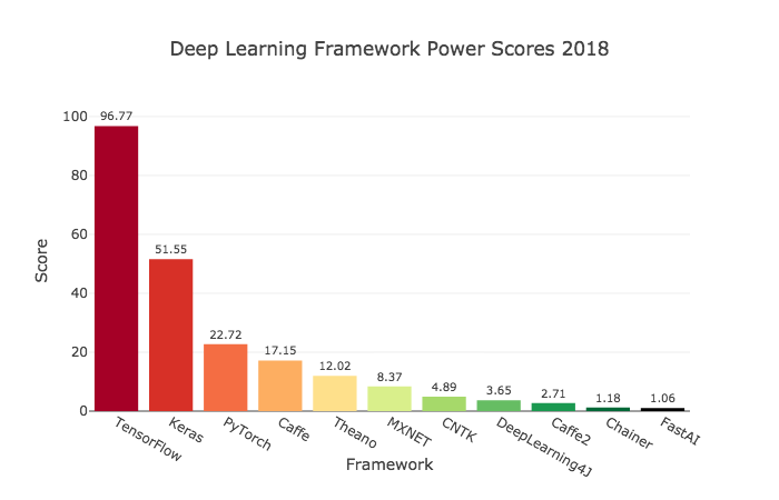
PyTorch, originally created by Facebook, is one of the most used frameworks, especially among researchers. The other most used framework are Tensorflow (created by Google) and Keras (an abstraction layer for multiple frameworks, including Tensorflow). PyTorch has gained a lot of popularity since its 1.0 release in 2018.

Why use Google Colab and GPUs?

Google Colab is a collaborative workspace based on Jupyter Notebook, that lets you use a Python environment on Google Cloud with GPUs, for FREE!

GPUs (Graphical Processing Units) are powerful chips that let you train and use neural networks much faster than CPUs. Having access to a GPU is very important for Deep Learning, as it can often make training more than 100x faster. It might not seem that huge at first, but state of the art neural nets can take days to train on common datasets, even with multiple powerful GPUs. On CPUs, it would take years.

Colab gives you access to a free Nvidia Tesla K80 (most of the time), which is a 1000€ graphics card with 24GB of VRAM.

/!\ IMPORTANT: Use a GPU Runtime

To use a GPU in Colab, go to Runtime -> Change Runtime Type -> Hardware Accelerator -> GPU.

Do this step before running any of the code below, otherwise you will have to run it again.

Importing libraries

For this lab, we only need PyTorch packages: “torch” and “torchvision”.

“torch“ contains the Deep Learning framework itself. “torchvision“ contains datasets, pre-trained models, and image manipulation functions.

#Import Pytorch
import torch
import torchvision

#Little commonly used shortcut
import torch.nn as nn

#We need the display function from IPython for Jupyter Notebook/Colab
from IPython.display import display

#A package to make beautiful progress bars :) 
from tqdm import tqdm_notebook

print(torch.__version__)

1.1.0

Downloading the data

使用最常用的mnist数据集，通过 torchvision.datasets 来下载数据集。

参数：

• root 下载的路径
• train 选择是训练集还是测试集
• download 是否下载
• 是否对数据进行变换，在torchvision.transforms中有许多变换函数

mnist_dataset = torchvision.datasets.MNIST(root = ".", train=True, download=True)

print(mnist_dataset[1])

Downloading http://yann.lecun.com/exdb/mnist/train-images-idx3-ubyte.gz to ./MNIST/raw/train-images-idx3-ubyte.gz


9920512it [00:01, 8710591.75it/s]                            


Extracting ./MNIST/raw/train-images-idx3-ubyte.gz

Done!
(<PIL.Image.Image image mode=L size=28x28 at 0x7FF31D48D7B8>, 0)

We see that each element is a tuple containing a PIL Image (Python Imaging Library) and a label (0 here).
We can visualize PIL images in Colab using the display function.

数据集中的每一个元素是一个tuple，第0位是PIL image, 第1位是label。
可以使用 display() 函数对图像进行显示

display(mnist_dataset[128][0])

Part 1: Looking at the data

Q1: Display 10 images with their label

显示十个图像和他们的label

for i in range(10):
  display(mnist_dataset[i][1],mnist_dataset[i][0])
# display(type(mnist_dataset[1][1]))

5

0

4

1

9

2

1

3

1

4

Q2: Display 10 images from a specific class

显示10个label为4的图像

count = 0
index = 0
while count != 10:
  if mnist_dataset[index][1] == 4:
    display(mnist_dataset[index][0],mnist_dataset[index][1])
    count += 1
  index += 1

4

4

4

4

4

4

4

4

4

4

Q3: Count the number of elements in each class

计算每一个标签有多少个元素

count = [0]*10
for element in mnist_dataset:
  count[element[1]] += 1
print(count)

[5923, 6742, 5958, 6131, 5842, 5421, 5918, 6265, 5851, 5949]

Part 2: Creating a Neural Network with torch.nn

我们使用经典的lenet网络

Q4: Implementing the network

All networks created with torch.nn are subclasses of nn.Module.

所有由 torch.nn 创建的网络都是 nn.Module 的子类。

为了创建一个网络，我们需要定义两个函数

• 在 __init__ 函数中，我们要定义网络所有需要的部件（layer），称其为网络的属性。
• 在 forward 函数中，我们要通过一个给定的输入来定义所有layer的顺序。(不太懂define-by-run)

class MyFirstNetwork(nn.Module):
  
  def __init__(self):
    super(MyFirstNetwork, self).__init__()
    
    ## MNIST images are 28x28 but LeNet5 expects 32x32
    ## -> we pad the images with zeroes
    self.padding = nn.ZeroPad2d(2)
    
    ## First convolution
    self.conv1 = nn.Conv2d(in_channels = 1, out_channels= 6 , kernel_size = 5)
    
    ## Second convolution
    self.conv2 = nn.Conv2d(in_channels=6,out_channels=16,kernel_size=5)
    
    ## Pooling (subsampling) layer
    self.maxpool = nn.MaxPool2d(2)
    
    ## Activation layer
    self.relu = nn.ReLU()
    
    ## Fully connected layers
    self.fc1 = nn.Linear(in_features = 400, out_features = 120)
    self.fc2 = nn.Linear(in_features=120,out_features=84)
    self.output = nn.Linear(in_features=84,out_features=10)
    
    ## Final activation layer
    self.softmax = nn.LogSoftmax(dim=1) # why log?
    
  def forward(self, x):
    
    ## Pad the input
    x = self.padding(x)
    
    ## First convolution + activation
    x = self.conv1(x)
    x = self.relu(x)
    
    ## First pooling
    x = self.maxpool(x)
    
    ## Second Convolution + activation
    x = self.conv2(x)
    x = self.relu(x)
    
    ## Second Pooling
    x = self.maxpool(x)
    
    ## "Flatten" the output to make it 1D
    x = x.view(-1, 16*5*5) # view 相当于np中的resize函数
    
    ## First full connection
    x = self.fc1(x)
    x = self.relu(x)
    
    ## Second full connection
    x = self.fc2(x)
    x = self.relu(x)
    
    ## Output layer
    x = self.output(x)
    y = self.softmax(x)
    
    return y

这里使用了 logSoftmax()，后面再配合NLLloss()。但是可以将这两部直接使用CrossEntropyLoss()代替(不再需要logsoftmax)

Testing our implementation

我们用数据集中的一个图像来测试我们刚刚搭建的网络

我们可以在前向传播的任意一点执行程序来debug我们的网络。 这是使用pytorch的众多好处之一。

动态计算意味着程序将按照我们编写命令的顺序进行执行。这种机制将使得调试更加容易，并且也使得我们将大脑中的想法转化为实际代码变得更加容易。而静态计算则意味着程序在编译执行时将先生成神经网络的结构，然后再执行相应操作。从理论上讲，静态计算这样的机制允许编译器进行更大程度的优化，但是这也意味着你所期望的程序与编译器实际执行之间存在着更多的代沟。这也意味着，代码中的错误将更加难以发现（比如，如果计算图的结构出现问题，你可能只有在代码执行到相应操作的时候才能发现它）

pytorch 运算单元为张量，就是N维矩阵，可以使用直接打印张量，也可以使用x.size()来查看大小。

## Create an instance of our network
net = MyFirstNetwork()

## Create a conversion function to convert PIL images into Tensors
convert = torchvision.transforms.ToTensor()

## Get our input image as a tensor. We add a dimension with "unsqueeze", because   不懂
## PyTorch is used to working with batches.
x = convert(mnist_dataset[0][0]).unsqueeze(0)

## Apply the network to the input
net(x)

tensor([[-2.3397, -2.2196, -2.3458, -2.2699, -2.2840, -2.2333, -2.3094, -2.2939,
         -2.3768, -2.3664]], grad_fn=<LogSoftmaxBackward>)

这里最后的grad_fn是pytorch里Variable中的特性，会在另外一篇文章中专门写一下pytorch的autograd。

Part 3: Training the network

Choosing a loss function and an optimizer

选择损失函数和优化器。

# Negative log likelihood loss
criterion = nn.NLLLoss()

# Stochastic Gradient Descent
# optimizer = torch.optim.SGD(net.parameters(), lr=0.01)
optimizer = torch.optim.Adam(net.parameters(),lr = 0.001)

Basic training bricks

网络的训练包括以下五步：

1. 计算前向传播

y = net(x)

1. 计算损失

loss = criterion(y, label)

1. 将梯度设置为0，否则梯度默认会累积（利于RNN计算）

optimizer.zero_grad()

1. 反向传播

loss.backward()

1. 在loss.backward()获得所有parameter的gradient，然后optimizer存了这些parameter的指针，step()根据这些parameter的gradient对parameter的值进行更新。 根据现在的梯度对参数进行更新

optimizer.step()

Q5: Creating a basic training loop

首先实现最简单的训练，让数据集中的元素一个个的经过网络。

## MODIFY THIS LINE IF THE TRAINING TAKES TOO LONG (MAX 60000)
SAMPLES_TO_USE = 4000

## NUMBER OF EPOCHS TO TRAIN
N_EPOCHS = 5

## Put the network in training mode
net.train()

for e in tqdm_notebook(range(N_EPOCHS), desc='Epochs'):
  
  running_loss = 0
  running_accuracy = 0
  
  for i in tqdm_notebook(range(SAMPLES_TO_USE), desc="Samples"):
    
    # Get a sample from the dataset
    sample = mnist_dataset[i]
    x = convert(sample[0]).unsqueeze(0)
    label = torch.tensor([sample[1]])

    y = net(x)
    loss = criterion(y, label)
    optimizer.zero_grad()
    loss.backward()
    optimizer.step()
    
    ## Compute some statistics
    with torch.no_grad():
      running_loss += loss.data
      running_accuracy += 1 if y.max(1)[1] == label else 0
    
  print("Training accuracy:", running_accuracy/SAMPLES_TO_USE)
  print("Training loss:", running_loss/SAMPLES_TO_USE)

HBox(children=(IntProgress(value=0, description='Epochs', max=5, style=ProgressStyle(description_width='initia…



HBox(children=(IntProgress(value=0, description='Samples', max=4000, style=ProgressStyle(description_width='in…


Training accuracy: 0.857
Training loss: tensor(0.4592)



HBox(children=(IntProgress(value=0, description='Samples', max=4000, style=ProgressStyle(description_width='in…


Training accuracy: 0.952
Training loss: tensor(0.1701)



HBox(children=(IntProgress(value=0, description='Samples', max=4000, style=ProgressStyle(description_width='in…


Training accuracy: 0.96275
Training loss: tensor(0.1162)



HBox(children=(IntProgress(value=0, description='Samples', max=4000, style=ProgressStyle(description_width='in…


Training accuracy: 0.9725
Training loss: tensor(0.0912)



HBox(children=(IntProgress(value=0, description='Samples', max=4000, style=ProgressStyle(description_width='in…


Training accuracy: 0.978
Training loss: tensor(0.0669)

Evaluating on a test set

使用测试集进行测试

#Get the MNIST test set
mnist_test_dataset = torchvision.datasets.MNIST(".", train=False, transform=convert, download=True)  # transform? convert?

print("Number of test images:", len(mnist_test_dataset))

#Put the network in eval mode
net.eval()

acc = 0
#Disable gradient computation for this (we do not need them, this will speed up testing)
with torch.no_grad():
  for img, label in tqdm_notebook(mnist_test_dataset):

    y = net(img.unsqueeze(0))

    if y.max(1)[1] == label:
      acc +=1

  print("Test Accuracy:", acc/len(mnist_test_dataset))

Number of test images: 10000



HBox(children=(IntProgress(value=0, max=10000), HTML(value='')))



Test Accuracy: 0.9566

Q6: Displaying a few random results from the test set

打印测试结果

HINT: to get the network output for a sample as a number, you can use:

net(convert(sample[0]).unsqueeze(0)).max(1)[1]

unsqueeze() 函数为在指定位置上增加维度，如一三行的tensor，则unsqueeze(0)后变为，一行三列的tensor。这里使用unsqueeze()是因为torch.nn不接受单独的样本，所以需要用其增加一个假维度。

max() 返回最大值，和其索引，参数为0则返回每列的最大值，1为返回每行的最大值

import random

mnist_test_dataset_PIL = torchvision.datasets.MNIST(".", train=False, download=True)

for i in range(10):
  output = net(convert(mnist_test_dataset_PIL[i][0]).unsqueeze(0)).max(1)[1]
  display(mnist_test_dataset_PIL[i][0],output)

tensor([7])

tensor([2])

tensor([1])

tensor([0])

Part 4: Creating a better training loop

Splitting between validation and training data

为数据集增加validation

## Load Dataset
mnist_dataset = torchvision.datasets.MNIST(".", train=True, transform=convert, download=True)

## Percentage of validation data
validation_split = 0.1

N_val_samples = round(validation_split * len(mnist_dataset))

## Split into two Subset
train_set, val_set = torch.utils.data.random_split(mnist_dataset, [len(mnist_dataset) - N_val_samples, N_val_samples])

# train and val are Subset objects
print(train_set,len(train_set))
print(val_set,len(val_set))

# Their sizes should be correct
len(train_set) + len(val_set) == len(mnist_dataset)

<torch.utils.data.dataset.Subset object at 0x7ff31c7957f0> 54000
<torch.utils.data.dataset.Subset object at 0x7ff31c795780> 6000





True

DataLoaders in PyTorch

In PyTorch, DataLoaders are tools that load batches of data from a Dataset (or any of its subclasses).
pytorch中的Dataloaders可以从数据集中以bath为单位装载数据。

Documentation on DataLoaders is here: https://pytorch.org/docs/stable/data.html

## This line creates a basic DataLoader from our mnist training set

## You can change options such as batch size, shuffling, number of workers...

BATCH_SIZE = 64

mnist_train_dl = torch.utils.data.DataLoader(train_set, batch_size=BATCH_SIZE, shuffle=True, num_workers=4) # num_workers 定义有几个cpu进行处理

Q7: Use the DataLoaders

Dataloder支持iterator

## Print the length of the dataloader
print(len(mnist_train_dl))
print(len(mnist_train_dl)==round((len(train_set)/BATCH_SIZE)))


## Print a batch

for batch in mnist_train_dl:
  print(batch[0])
  break

844
True
tensor([[[[0., 0., 0.,  ..., 0., 0., 0.],
          [0., 0., 0.,  ..., 0., 0., 0.],
          [0., 0., 0.,  ..., 0., 0., 0.],
          ...,
          [0., 0., 0.,  ..., 0., 0., 0.],
          [0., 0., 0.,  ..., 0., 0., 0.],
          [0., 0., 0.,  ..., 0., 0., 0.]]],


        [[[0., 0., 0.,  ..., 0., 0., 0.],
          [0., 0., 0.,  ..., 0., 0., 0.],
          [0., 0., 0.,  ..., 0., 0., 0.],
          ...,
          [0., 0., 0.,  ..., 0., 0., 0.],
          [0., 0., 0.,  ..., 0., 0., 0.],
          [0., 0., 0.,  ..., 0., 0., 0.]]],


        [[[0., 0., 0.,  ..., 0., 0., 0.],
          [0., 0., 0.,  ..., 0., 0., 0.],
          [0., 0., 0.,  ..., 0., 0., 0.],
          ...,
          [0., 0., 0.,  ..., 0., 0., 0.],
          [0., 0., 0.,  ..., 0., 0., 0.],
          [0., 0., 0.,  ..., 0., 0., 0.]]],


        ...,


        [[[0., 0., 0.,  ..., 0., 0., 0.],
          [0., 0., 0.,  ..., 0., 0., 0.],
          [0., 0., 0.,  ..., 0., 0., 0.],
          ...,
          [0., 0., 0.,  ..., 0., 0., 0.],
          [0., 0., 0.,  ..., 0., 0., 0.],
          [0., 0., 0.,  ..., 0., 0., 0.]]],


        [[[0., 0., 0.,  ..., 0., 0., 0.],
          [0., 0., 0.,  ..., 0., 0., 0.],
          [0., 0., 0.,  ..., 0., 0., 0.],
          ...,
          [0., 0., 0.,  ..., 0., 0., 0.],
          [0., 0., 0.,  ..., 0., 0., 0.],
          [0., 0., 0.,  ..., 0., 0., 0.]]],


        [[[0., 0., 0.,  ..., 0., 0., 0.],
          [0., 0., 0.,  ..., 0., 0., 0.],
          [0., 0., 0.,  ..., 0., 0., 0.],
          ...,
          [0., 0., 0.,  ..., 0., 0., 0.],
          [0., 0., 0.,  ..., 0., 0., 0.],
          [0., 0., 0.,  ..., 0., 0., 0.]]]])

Q8: Create a DataLoader for the validation set

同样的方式给validation使用dataloader

mnist_val_dl = torch.utils.data.DataLoader(val_set, batch_size=BATCH_SIZE, shuffle=True, num_workers=4)

Using a GPU

为了让运算在GPU上进行，我们需要用cuda()函数将batch移动到GPU上。

batch = torch.Tensor(next(iter(mnist_train_dl))[0])

batch = batch.cuda()

同样的，使用cuda()将网络移植到GPU上

## Create an instance of our network
net = MyFirstNetwork()

## Move it to the GPU
net = net.cuda()

测试一下

output = net(batch)

print(output)

tensor([[-2.2496, -2.2465, -2.3473, -2.3269, -2.3198, -2.3962, -2.2808, -2.3959,
         -2.1621, -2.3246],
        [-2.2491, -2.2417, -2.3421, -2.3355, -2.3201, -2.3880, -2.2916, -2.3951,
         -2.1630, -2.3226],
        [-2.2500, -2.2550, -2.3535, -2.3268, -2.3125, -2.3907, -2.2792, -2.3997,
         -2.1548, -2.3282],
        [-2.2553, -2.2545, -2.3434, -2.3200, -2.3127, -2.3953, -2.2880, -2.4040,
         -2.1455, -2.3334],
        [-2.2513, -2.2498, -2.3574, -2.3193, -2.3051, -2.3952, -2.2874, -2.3989,
         -2.1557, -2.3307],
        [-2.2517, -2.2439, -2.3512, -2.3348, -2.3182, -2.3850, -2.2847, -2.3965,
         -2.1562, -2.3279],
        [-2.2512, -2.2551, -2.3502, -2.3282, -2.3064, -2.3870, -2.2891, -2.3970,
         -2.1566, -2.3285],
        [-2.2505, -2.2513, -2.3561, -2.3258, -2.3109, -2.3911, -2.2852, -2.3973,
         -2.1542, -2.3281],
        [-2.2516, -2.2497, -2.3511, -2.3215, -2.3018, -2.3900, -2.2891, -2.4002,
         -2.1600, -2.3345],
        [-2.2457, -2.2440, -2.3601, -2.3254, -2.3183, -2.3858, -2.2883, -2.3939,
         -2.1705, -2.3158],
        [-2.2511, -2.2438, -2.3493, -2.3325, -2.3185, -2.3958, -2.2782, -2.3907,
         -2.1639, -2.3255],
        [-2.2507, -2.2528, -2.3525, -2.3236, -2.3119, -2.3939, -2.2798, -2.4015,
         -2.1570, -2.3267],
        [-2.2571, -2.2424, -2.3539, -2.3254, -2.3203, -2.3893, -2.2838, -2.4012,
         -2.1549, -2.3223],
        [-2.2486, -2.2467, -2.3522, -2.3259, -2.3173, -2.3868, -2.2981, -2.3925,
         -2.1630, -2.3172],
        [-2.2514, -2.2511, -2.3469, -2.3301, -2.3107, -2.3830, -2.2960, -2.3962,
         -2.1551, -2.3286],
        [-2.2458, -2.2469, -2.3488, -2.3333, -2.3165, -2.3888, -2.2849, -2.3978,
         -2.1654, -2.3208],
        [-2.2413, -2.2510, -2.3632, -2.3166, -2.3084, -2.3880, -2.2906, -2.3988,
         -2.1659, -2.3255],
        [-2.2451, -2.2529, -2.3573, -2.3157, -2.3164, -2.3888, -2.2934, -2.3992,
         -2.1548, -2.3268],
        [-2.2503, -2.2504, -2.3439, -2.3264, -2.3140, -2.3946, -2.2888, -2.3939,
         -2.1602, -2.3264],
        [-2.2522, -2.2513, -2.3503, -2.3258, -2.3054, -2.3835, -2.2912, -2.4010,
         -2.1545, -2.3346],
        [-2.2451, -2.2426, -2.3602, -2.3312, -2.3160, -2.3904, -2.2852, -2.3970,
         -2.1636, -2.3186],
        [-2.2495, -2.2419, -2.3558, -2.3262, -2.3133, -2.3906, -2.2856, -2.4010,
         -2.1629, -2.3231],
        [-2.2455, -2.2500, -2.3498, -2.3308, -2.3121, -2.3836, -2.2918, -2.3926,
         -2.1739, -2.3163],
        [-2.2518, -2.2392, -2.3594, -2.3274, -2.3155, -2.3858, -2.2901, -2.3956,
         -2.1661, -2.3178],
        [-2.2492, -2.2485, -2.3483, -2.3257, -2.3169, -2.3943, -2.2902, -2.3956,
         -2.1545, -2.3272],
        [-2.2535, -2.2451, -2.3540, -2.3294, -2.3189, -2.3858, -2.2851, -2.3972,
         -2.1586, -2.3218],
        [-2.2484, -2.2553, -2.3578, -2.3296, -2.3079, -2.3865, -2.2841, -2.3963,
         -2.1630, -2.3197],
        [-2.2515, -2.2416, -2.3507, -2.3306, -2.3198, -2.3834, -2.2939, -2.3965,
         -2.1601, -2.3208],
        [-2.2530, -2.2472, -2.3479, -2.3281, -2.3179, -2.3893, -2.2871, -2.3980,
         -2.1535, -2.3282],
        [-2.2462, -2.2389, -2.3614, -2.3256, -2.3219, -2.3898, -2.2890, -2.4019,
         -2.1572, -2.3195],
        [-2.2521, -2.2456, -2.3462, -2.3293, -2.3137, -2.3905, -2.2852, -2.3963,
         -2.1581, -2.3327],
        [-2.2556, -2.2474, -2.3382, -2.3331, -2.3116, -2.3897, -2.2867, -2.3988,
         -2.1578, -2.3303],
        [-2.2482, -2.2566, -2.3535, -2.3242, -2.3099, -2.3876, -2.2933, -2.3972,
         -2.1568, -2.3220],
        [-2.2458, -2.2426, -2.3591, -2.3288, -2.3218, -2.3814, -2.2931, -2.3931,
         -2.1645, -2.3184],
        [-2.2469, -2.2424, -2.3518, -2.3288, -2.3185, -2.3942, -2.2822, -2.4004,
         -2.1636, -2.3212],
        [-2.2479, -2.2457, -2.3571, -2.3189, -2.3172, -2.3914, -2.2910, -2.3971,
         -2.1604, -2.3231],
        [-2.2475, -2.2499, -2.3540, -2.3260, -2.3162, -2.3965, -2.2786, -2.3959,
         -2.1628, -2.3223],
        [-2.2510, -2.2464, -2.3442, -2.3314, -2.3124, -2.3877, -2.2909, -2.3980,
         -2.1572, -2.3303],
        [-2.2508, -2.2410, -2.3470, -2.3257, -2.3149, -2.3994, -2.2841, -2.4011,
         -2.1610, -2.3256],
        [-2.2505, -2.2426, -2.3576, -2.3258, -2.3186, -2.3865, -2.2879, -2.3969,
         -2.1624, -2.3206],
        [-2.2464, -2.2476, -2.3491, -2.3319, -2.3155, -2.3912, -2.2847, -2.3945,
         -2.1649, -2.3229],
        [-2.2513, -2.2422, -2.3560, -2.3274, -2.3174, -2.3853, -2.2955, -2.3945,
         -2.1575, -2.3225],
        [-2.2468, -2.2480, -2.3572, -2.3199, -2.3168, -2.3960, -2.2866, -2.3976,
         -2.1583, -2.3234],
        [-2.2489, -2.2562, -2.3495, -2.3251, -2.3133, -2.3860, -2.2914, -2.3960,
         -2.1535, -2.3296],
        [-2.2502, -2.2405, -2.3475, -2.3375, -2.3183, -2.3872, -2.2880, -2.3920,
         -2.1669, -2.3201],
        [-2.2485, -2.2459, -2.3606, -2.3223, -2.3153, -2.3864, -2.2832, -2.3979,
         -2.1652, -2.3236],
        [-2.2530, -2.2487, -2.3475, -2.3211, -2.3158, -2.3915, -2.2929, -2.4006,
         -2.1516, -2.3281],
        [-2.2560, -2.2425, -2.3430, -2.3359, -2.3174, -2.3909, -2.2819, -2.3926,
         -2.1589, -2.3303],
        [-2.2454, -2.2492, -2.3632, -2.3174, -2.3149, -2.3910, -2.2952, -2.3935,
         -2.1570, -2.3232],
        [-2.2490, -2.2511, -2.3444, -2.3312, -2.3069, -2.3892, -2.2841, -2.3962,
         -2.1602, -2.3368],
        [-2.2544, -2.2470, -2.3511, -2.3255, -2.3141, -2.3874, -2.2884, -2.4005,
         -2.1542, -2.3277],
        [-2.2503, -2.2418, -2.3410, -2.3357, -2.3193, -2.3898, -2.2904, -2.3934,
         -2.1664, -2.3200],
        [-2.2456, -2.2445, -2.3542, -2.3286, -2.3163, -2.3860, -2.2909, -2.3977,
         -2.1674, -2.3173],
        [-2.2480, -2.2516, -2.3516, -2.3293, -2.3165, -2.3851, -2.2886, -2.3963,
         -2.1582, -2.3239],
        [-2.2528, -2.2583, -2.3459, -2.3284, -2.3144, -2.3838, -2.2924, -2.3973,
         -2.1534, -2.3223],
        [-2.2539, -2.2382, -2.3514, -2.3291, -2.3191, -2.3879, -2.2878, -2.3955,
         -2.1599, -2.3267],
        [-2.2547, -2.2498, -2.3432, -2.3298, -2.3157, -2.3909, -2.2847, -2.3966,
         -2.1607, -2.3225],
        [-2.2485, -2.2391, -2.3439, -2.3377, -2.3207, -2.3891, -2.2897, -2.3941,
         -2.1662, -2.3196],
        [-2.2505, -2.2533, -2.3467, -2.3262, -2.3103, -2.3942, -2.2868, -2.3975,
         -2.1565, -2.3280],
        [-2.2508, -2.2545, -2.3510, -2.3253, -2.3084, -2.3834, -2.2950, -2.3988,
         -2.1516, -2.3313],
        [-2.2537, -2.2451, -2.3405, -2.3270, -2.3199, -2.3960, -2.2837, -2.3978,
         -2.1605, -2.3254],
        [-2.2535, -2.2411, -2.3562, -2.3289, -2.3218, -2.3815, -2.2918, -2.3947,
         -2.1615, -2.3177],
        [-2.2496, -2.2454, -2.3588, -2.3243, -2.3090, -2.3904, -2.2906, -2.3978,
         -2.1585, -2.3257],
        [-2.2516, -2.2559, -2.3545, -2.3239, -2.3047, -2.3863, -2.2907, -2.3990,
         -2.1581, -2.3242]], device='cuda:0', grad_fn=<LogSoftmaxBackward>)

Q9: Our new training/validation loop

启用新的训练，这次使用了dataloader并且增加了validatio。

##RE-RUN THIS CODE TO GET A "NEW" NETWORK

LEARNING_RATE = 0.001
MOMENTUM = 0

## Create an instance of our network
net = MyFirstNetwork()

## Move it to the GPU
net = net.cuda()

# Negative log likelihood loss
criterion = nn.NLLLoss()

# Stochastic Gradient Descent
optimizer = torch.optim.SGD(net.parameters(), lr=LEARNING_RATE, momentum=MOMENTUM)

## NUMBER OF EPOCHS TO TRAIN
N_EPOCHS = 20

epoch_loss, epoch_acc, epoch_val_loss, epoch_val_acc = [], [], [], []



for e in tqdm_notebook(range(N_EPOCHS), desc='Epochs'):
  
  
  ### TRAINING LOOP
  running_loss = 0
  running_accuracy = 0
  
  ## Put the network in training mode
  net.train()
  
  for i, batch in enumerate(tqdm_notebook(mnist_train_dl, desc="Training Batches")):
    
    # Get a batch from the dataloader
    x = batch[0]
    labels = batch[1]
    
    # move the batch to GPU
    x = x.cuda()
    labels = labels.cuda()

    # Compute the network output
    y = net(x)
    
    # Compute the loss
    loss = criterion(y, labels)
    
    # Reset the gradients
    optimizer.zero_grad()
    
    # Compute the gradients
    loss.backward()
    
    # Apply one step of the descent algorithm to update the weights
    optimizer.step()
    
    ## Compute some statistics
    with torch.no_grad():
      running_loss += loss.item()
      running_accuracy += (y.max(1)[1] == labels).sum().item()
    
  print("Training accuracy:", running_accuracy/float(len(train_set)),
        "Training loss:", running_loss/float(len(train_set)))
  
  epoch_loss.append(running_loss/len(train_set))
  epoch_acc.append(running_accuracy/len(train_set))
  
  ### VALIDATION LOOP
  ## Put the network in validation mode
  net.eval()
  
  running_val_loss = 0
  running_val_accuracy = 0
  
  for i, batch in enumerate(tqdm_notebook(mnist_val_dl, desc="Validation Batches")): 
    labels = batch[1].cuda()
    answer = net(batch[0].cuda())
    val_loss = criterion(answer, labels)
    with torch.no_grad():
      running_val_accuracy += (answer.max(1)[1] == labels).sum().item()
      running_val_loss += val_loss.item()
    
  epoch_val_loss.append(running_val_loss/float(len(val_set)))
  epoch_val_acc.append(running_val_accuracy/float(len(val_set)))
  print(running_val_loss/float(len(val_set)))
  print(running_val_accuracy/float(len(val_set)))

HBox(children=(IntProgress(value=0, description='Epochs', max=20, style=ProgressStyle(description_width='initi…



HBox(children=(IntProgress(value=0, description='Training Batches', max=844, style=ProgressStyle(description_w…


Training accuracy: 0.09942592592592593 Training loss: 0.036009652340853654



HBox(children=(IntProgress(value=0, description='Validation Batches', max=94, style=ProgressStyle(description_…


0.036064300735791525
0.09666666666666666



。。。。。。。。。。。。。。。。。。。。。。。。。

HBox(children=(IntProgress(value=0, description='Training Batches', max=844, style=ProgressStyle(description_w…


Training accuracy: 0.9074444444444445 Training loss: 0.004941175849211436



HBox(children=(IntProgress(value=0, description='Validation Batches', max=94, style=ProgressStyle(description_…


0.00460548147186637
0.9078333333333334

Q10: Making a graph with training/validation accuracy and loss

可视化训练结果

import matplotlib.pyplot as plt
import numpy as np

x_axis = list(range(1,21))
plt.title('loss')
plt.xlabel = 'Epoch'
plt.ylabel = 'Loss'
plt.plot(x_axis,epoch_loss,label='Training')
plt.plot(x_axis,epoch_val_loss,label='Validation')
plt.legend(loc='upper right')
plt.show()

Q11: Evaluate our network on the test set (on GPU)

同样使用dataloder进行测试

#Get the MNIST test set
mnist_test_dataset = torchvision.datasets.MNIST(".", train=False, transform=convert, download=True)
mnist_test_dl = torch.utils.data.DataLoader(mnist_test_dataset, batch_size=BATCH_SIZE, shuffle=True, num_workers=4)
running_test_accuracy = 0
running_test_loss = 0
with torch.no_grad():
    for i, batch in enumerate(tqdm_notebook(mnist_test_dl, desc="Test Batches")): 
      labels = batch[1].cuda() 
      answer = net(batch[0].cuda())
      # print(answer.max(1)[1])
      # print(batch[1])
      running_test_accuracy += (answer.max(1)[1] == labels).sum().item()
      running_test_loss = criterion(answer, labels)

    running_test_accuracy = 100. * running_test_accuracy/len(mnist_test_dataset)
print(running_test_loss)
print(running_test_accuracy)

HBox(children=(IntProgress(value=0, description='Test Batches', max=157, style=ProgressStyle(description_width…



tensor(0.1383, device='cuda:0')
91.49

(OPTIONAL) Part 5: Cats vs Dogs with a torchvision network

To test our skills on a new dataset, we will work on the famous Dogs vs Cats Kaggle dataset.

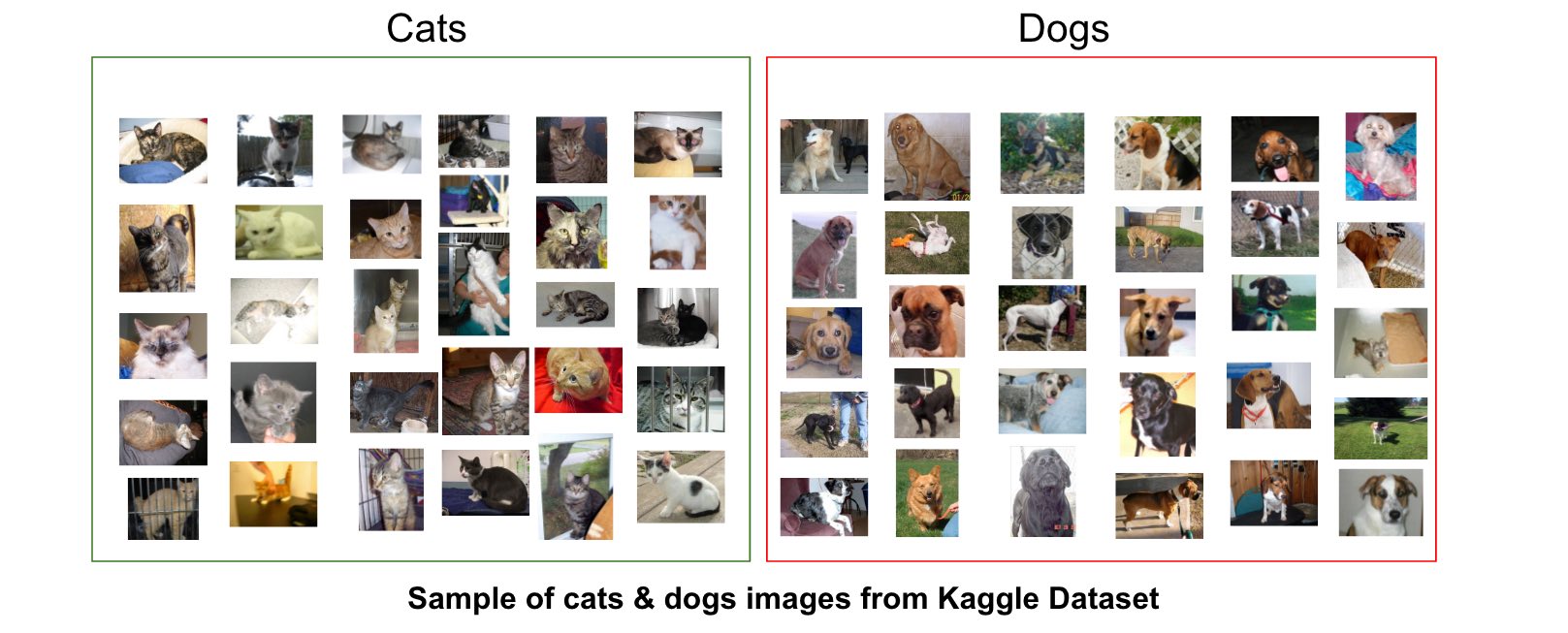
Kaggle is a website that hosts machine learning/data science competitions. Check it out! https://www.kaggle.com/

Downloading the data

First, go to the Kaggle website and create an account.

Then go to your account, click on Create New API Token - It will download kaggle.json file on your machine.

Upload the kaggle.json file using this code:

! pip install -q kaggle

from google.colab import files

files.upload()

 <input type="file" id="files-65ec0027-1fa8-4b32-bc71-a4d5bc6f7c57" name="files[]" multiple disabled />
 <output id="result-65ec0027-1fa8-4b32-bc71-a4d5bc6f7c57">
  Upload widget is only available when the cell has been executed in the
  current browser session. Please rerun this cell to enable.
  </output>
  <script src="/nbextensions/google.colab/files.js"></script> 


Saving kaggle (1).json to kaggle (1).json





{'kaggle (1).json': b'{"username":"wangzeyao","key":"6d3445d98da97c96f236cda74bbd2105"}'}

Download the dogs vs cats dataset using this code:

! mkdir ~/.kaggle

! cp kaggle.json ~/.kaggle/

! chmod 600 ~/.kaggle/kaggle.json

! kaggle competitions download -c dogs-vs-cats

mkdir: cannot create directory ‘/root/.kaggle’: File exists
401 - Unauthorized

Extract the archives:

! rm -rf test1 train

! unzip -q train.zip

! unzip -q test1.zip

Put the data in separate directories:

! mkdir train/cats
! mkdir train/dogs
! mv train/cat.* train/cats
! mv train/dog.* train/dogs

Q12: Load the data

Using ImageFolder from torchvision (https://pytorch.org/docs/stable/torchvision/datasets.html#imagefolder), load the dataset.

The training set is in the “train” directory.

### YOUR CODE HERE

Q13: Display a few images

As before, display a few images with the display function. You can see that these images have varying sizes.

### YOUR CODE HERE

Using a torchvision model

torchvision has a repository of popular models ready to use for diverse computer vision tasks (classification, segmentation,…)

https://pytorch.org/docs/stable/torchvision/models.html#classification

## You can change the model if you want
net = torchvision.models.resnet18()

print(net)

## torchvision models are meant to be used on imagenet (1000 classes)
## since we only have two classes, we need to modify the last layer

net.fc = nn.Linear(512,2)

Q14: Resize the images on the fly using torchvision transforms

We can see from the documentation that torchvision models expect at least 244x244 images.

1. Using torchvision.transforms, create a new ImageFolder dataset with on-the-fly resizing of images.

2. Split this Dataset into training and validation sets, as before.

3. Create a DataLoader for each set as well, just like before.

### YOUR CODE HERE

Q15: Training the model

Write the training loop. You should be able to pretty much copy-paste the one from Q9.

LEARNING_RATE = 0.001

## Move model to the GPU
net = net.cuda()

# Negative log likelihood loss
criterion = nn.NLLLoss()

# Stochastic Gradient Descent
optimizer = torch.optim.Adam(net.parameters(), lr=LEARNING_RATE)

### YOUR CODE HERE

Q16: Test the network

Compute some predictions on the test set.

### YOUR CODE HERE

Q17: Going further

Try different networks from torchvision, and different parameters. The winner of the competition got more than 98% accuracy. How much can you get?

Data augmentation (modifying your input data to make “more” of it) is a huge thing in deep learning. Try some techniques such as random cropping and rotation using torchvision transforms in your Dataset objects!

PyTorch has a lot of tutorials to get you started: https://pytorch.org/tutorials/index.html

Have fun!